When considering many turns of an accelerator lattice, we observe the behaviour of a beam envelope. Hill's equation's are second order differential equations for a system with periodic focussing properties. The motion has a variable spring constant $k(s)$ which depends on the magnetic properties of the accelerator ring. If the ring has periodicity L, then so does the function $k(s)$:
\begin{equation}k(s+L) ~=~ k(s)\end{equation}
From this we can expect something similar to harmonic oscillation where the frequency and amplitude depend on the location in the accelerator ring, and show periodicity similar to that of the function $k(s)$.
The Courant-Snyder formalism assumes a solution of Hill's equation inspired by this intuition on position dependent amplitude and phase, to provide us with a set of auxiliary functions that allow us to extract the maximum information from Hill's equations. Thus we use the ansatz:
\begin{equation}x(s) ~=~ \sqrt{\epsilon \beta(s) }~ cos ( \psi (s) + \psi_0).\end{equation}
$\beta(s)$ is a position dependent amplitude, $\psi(s)$ is a position dependent phase, and $\epsilon$ is a constant known as the emittance. As Hill's equation is linear the emittance does not appear in it. $\beta(s)$ is the important variable in the Courant-Snyder formalism. Having many names such as the beta function and the beam envelope function, it has the physical meaning of amplitude, which is dependent on the position along the accelerator. It represents the focussing properties of an accelerator lattice, a small $\beta$ represents a tightly focussed lattice. We note that $\beta(s+L) = \beta(s)$.
Taking derivatives of the Courant-Snyder ansatz and substituting into the equation of motion, we get two terms; one proportional to cos and the other proportional to sin. We obtain two differential equations:
\begin{equation}\frac{1}{2} (\beta \beta'' - \frac{1}{2} \beta'^2) - \beta^2 \psi^2 + \beta^2k ~=~0,\end{equation}
\begin{equation}\beta'\psi' + \beta\psi'' ~=~ 0.\end{equation}
The latter may be integrated as:
\begin{equation} \beta'\phi' + \beta\psi'' ~=~ (\beta\psi')'. \end{equation}
We may choose the integration constant to be 1, $\beta\psi'=1$. The result for the phase function is thus:
\begin{equation}
\psi(s) ~=~ \int\limits_0^s \frac{ds}{\beta(s)},
\end{equation}
a position dependent phase, which is related to an integration of the beta function along the beam line. Knowing the beta function means that we may compute the phase function. We can eliminate the phase function from the first Courant-Snyder differential equation, to obtain a differential equation for the beta function:
\begin{equation} \frac{1}{2} \beta \beta'' - \frac {1}{4}\beta'^2 + \beta^2k ~=~1 \end{equation}
Thus we see that $\beta$ is determined by the distribution of focussing strengths along the accelerator, though we do not solve this equation in practice. We define two functions that, along with $\beta$, are called the lattice, or sometimes TWISS functions:
\begin{equation} \alpha(s) ~=~ \frac{-1}{2} \frac{d\beta(s)}{ds}, \end{equation}
and
\begin{equation} \gamma(s) ~=~ \frac{1+\alpha(s)^2}{\beta(s)}. \end{equation}
Once the lattice functions are known, the motion of a single particle through the lattice is completely defined in specifying the emittance and initial phase factor of the particle.
After some algebra we see that
\begin{equation} \epsilon ~=~ \gamma x^2 + 2 \alpha x x' + \beta x'^2. \end{equation}
Original Paper
E.D. Courant and H.S. Snyder, Ann. Phys. 3, 1 (1958)
Adapted from
[1] S. Y. Lee, Accelerator Physics, Second Edition, World Scientific, 2007
[2] H. Weidemann. Particle Accelerator Physics I: Basic Principles and Linear Beam
Dynamics. Springer, 1999
[3] R. Appleby, Beam Dynamics, Cockcroft Lectures 2011
Showing posts with label Accelerator Physics. Show all posts
Showing posts with label Accelerator Physics. Show all posts
Thursday, 19 December 2013

2. Hill's Equations
Hill's equations; linearised second order differential equations for the transverse variables $x$ and $y$ in dipole and quadrupole fields within an accelerator are :
\begin{equation}x(s)'' + \left( k(s) + \frac{1}{\rho(s)^2} \right) x(s) ~=~ 0,\end{equation}
and
\begin{equation}y(s)'' - k(s) y ~=~ 0.\end{equation}
where $\rho = const$ and $k=const$ . Hills equations may be written compactly;
\begin{equation}x''+ K \cdot x ~=~ 0.\end{equation}
Where $K = k, K = (k + \frac{1}{\rho^2})$; if we write K for the constant and assume that it is constant over the accelerator, these equations appear similar to that of the a harmonic oscillator.
\begin{equation}x(s)'' + \left( k(s) + \frac{1}{\rho(s)^2} \right) x(s) ~=~ 0,\end{equation}
and
\begin{equation}y(s)'' - k(s) y ~=~ 0.\end{equation}
where $\rho = const$ and $k=const$ . Hills equations may be written compactly;
\begin{equation}x''+ K \cdot x ~=~ 0.\end{equation}
Where $K = k, K = (k + \frac{1}{\rho^2})$; if we write K for the constant and assume that it is constant over the accelerator, these equations appear similar to that of the a harmonic oscillator.
1. Coordinates
We begin by defining a curved coordinate system, the curvature $\rho$ produced by a local dipole field, and the path length along the design trajectory is $s$. The position of a particle in these coordinates is:

\begin{equation} r ~=~ \rho + x. \end{equation}
These coordinates represent deviations with respect to the ideal design orbit, we assume these deviations to be small; in reality $x$ is in the of order mm. We use the positions $x$ and $y$, and their slopes $x' = \frac{dx}{ds}$ and $y' = \frac{dy}{ds}$.
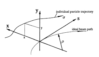
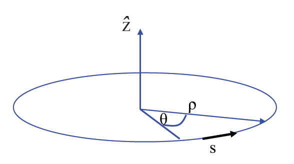
Circular coordinate system [1]
\begin{equation} \vec{R} ~=~ r \vec{x} + y \vec{z}, \end{equation}
where\begin{equation} r ~=~ \rho + x. \end{equation}
These coordinates represent deviations with respect to the ideal design orbit, we assume these deviations to be small; in reality $x$ is in the of order mm. We use the positions $x$ and $y$, and their slopes $x' = \frac{dx}{ds}$ and $y' = \frac{dy}{ds}$.

Circular coordinate system [2]
References
[1] R. Appleby. Beam Dynamics. Cockcroft Lectures 2011
[2] H. Weidemann. Particle Accelerator Physics I: Basic Principles and Linear Beam
Dynamics. Springer, 1999
Tuesday, 11 June 2013
The Three Gables
In this instance our Three Gables refer to men of the mathematical world rather than a house in Harrow Weald; Newton, Hamilton and Lagrange.
Let us take the example of the simple pendulum and the three mathematicians' approaches to finding the equations of motion for this dynamical system. The pendulum weight has mass $m$, $\mathbf{x}$ denotes its position vector, $\dot{\mathbf{x}}$ its velocity vector (i.e. $\frac{d(\mathbf{x})}{dt}=\dot{\mathbf{x}}$) and $\mathbf{p}$ is the momentum vector of the pendulum mass.
Approaches
Newton: Relate a force $\mathbf{F}(\mathbf{x}, \dot{\mathbf{x}}, t)$ to the resulting motion using Newton's 2nd law: $F=ma$ or more appropriately $$\frac{d}{dt}m\dot{\mathbf{x}} = \mathbf{F}(\mathbf{x}, \dot{\mathbf{x}}, t).$$
Lagrange: Construct the Lagrangian function $\mathcal{L}(q, \dot{q},t)$ which can normally be given by $\mathcal{L} = T - V$ where $T$ and $V$ are the kinetic and potential energy of the system respectively. The equations of motion are given by the Euler-Lagrange equation: $$ \frac{d\mathcal{L}}{dq_i} - \frac{d}{dt} \left( \frac{d\mathcal{L}}{d\dot{q}_i} \right) = 0.$$
Hamilton: Construct the Hamiltonian function $H(\mathbf{x}, \mathbf{p},t)$, which is a function of a set of conjugate variable pairs. The Hamiltonian contains the dynamics of the system and Hamilton's equations provide the equations of motion: $$ \frac{d\mathbf{x}_i}{dt} = \frac{\partial H}{\partial \mathbf{x}_i}, $$ $$ \frac{d\mathbf{p}_i}{dt} = \frac{\partial H}{\partial \mathbf{p}_i}. $$
1: Newtonian Mechanics
This is the familiar method for most of us. I have dropped the bold font for vectors from here on.
The force on the pendulum mass is given by $F = -kx$ where $k$ is a constant given by $$k = \omega^2 m $$. Thus we can write $$F=-\omega^2 m.$$
Using Newton's 2nd law we get the equation of motion: $$ m \frac{d}{dt} \dot{x} = -m \omega^2 x, $$ which is equivalent to $$ \frac{d^2 x}{dt^2} = - \omega^2x.$$
The solution to this equation is the standard, two constant oscillatory equation: $$ x(t) = x_0 sin(\omega t + \phi_0)$$ where $x_0$ and $\phi_0$ are constants determined by the inital values of $x(t)$ and $\dot{x}(t)$.
2: Lagrangian Mechanics
The pendulum mass has a kinetic energy: $$T = \frac{1}{2} m \dot{x}^2 $$ and a potential energy given by $$V = \frac{1}{2}m \omega^2 x^2.$$
The Lagrangian in this case may be found using $\mathcal{L} = T-V$: $$\mathcal{L} = T-V = \frac{1}{2} m \dot{x}^2 - \frac{1}{2}m \omega^2 x^2. $$
Using the Euler-Lagrange equation: $$ \frac{d\mathcal{L}}{dx_i} - \frac{d}{dt}\left( \frac{d\mathcal{L}}{d\dot{x}_i}\right) = 0.$$
we can do this step by step:
$$ \frac{d\mathcal{L}}{dx_i} = -\omega^2 mx,$$
and:
$$ \frac{d\mathcal{L}}{d\dot{x}_i}=m\dot{x}.$$
Substituting into the Euler-Lagrange equation we have:
$$-\omega^2 m x - \frac{d}{dt}(m\dot{x}) = 0$$
which is equivalent to:
$$\frac{d^2 x}{dt^2} = -\omega^2 x.$$
Which unsurprisingly is equivalent to our Newtonian formulation and has the same standard oscillatory solution.
3: Hamiltonian
Here we need to use the conjugate pair of position $x_i$ and momentum $p_i$. Given the Lagrangian $\mathcal{L}$, the conjugate momentum and Hamiltonian can be derived as follows:
$$p_i = \frac{\partial \mathcal{L}}{\partial \dot{q}_i} = \frac{\partial \mathcal{L}}{\partial \dot{x}_i} = m\dot{x},$$
$$H = \sum_i \dot{q_i}{p_i} - \mathcal{L} = \sum_i \dot{x}_i p_i - \mathcal{L},$$
which leads to:
$$H = \dot{x}p_x - \mathcal{L} = m\dot{x}^2 - \mathcal{L},$$
and finally we have the Hamiltonian:
$$H = \frac{p^2_x}{2m} + \frac{1}{2}m \omega^2 x^2.$$
Using Hamilton's equations:
$$\frac{dx}{dt} = \frac{\partial H}{\partial p_x} = \frac{p_x}{m}, $$
$$\frac{d p_x}{dt}=-\frac{\partial H}{\partial x} = -m \omega^2 x. $$
Note that the last equation is equivalent to Newton's second law.
Remarks
Using Newtonian mechanics, given the function $\mathbf{F}$, we derive the equations of motion, which must be solved to give the explicit dependence of position $x$ (and thus velocity $\dot{x}$) on the independent parameter $t$.
The physics is constructing the form of $\mathbf{F}$ for a gvien system.
Using Lagrangian mechanics the variables $q_i$ can be any convenient set of parameters that describe the system state. We treat $q_i$ and $\dot{q}_i$ as independent variables, despite the fact that they are not. For $n$ degrees of freedom, the Euler-Lagrange equations give us $n$ second-order differential equations.
The physics is constructing the form of $\mathcal{L}$ for a given system.
Using Hamiltonian mechanics a set of conjugate variables that describe the system state must be carefully chosen. We treat the conjugate pair $x,p_x$ as independent variables despite the fact that they are related. For $n$ degrees of freedom, Hamilton's equations give us $2n$ first-order differential equations. Representing the dynamics using first-order differential equations has some advantages when considering linear methods.
The Hamiltonian is conserved if the independent variable does not appear explicitly in the Hamiltonian. This can be shown:
$$\frac{dH}{dt} = \frac{\partial H}{\partial x}\frac{dx}{dt} + \frac{\partial H}{\partial p_x}\frac{d p_x}{dt} + \frac{\partial H}{\partial t}$$
substituting in Hamilton's equations the first two terms cancel:
$$\frac{dH}{dt} = \frac{\partial H}{\partial x}\frac{\partial H}{\partial p_x} + \frac{\partial H}{\partial p_x}\frac{\partial H}{\partial x} + \frac{\partial H}{\partial t} = \frac{\partial H}{\partial t}.$$
If the Hamiltonian does not depend explicitly on $t$, then the Hamiltonian is conserved:
$$\frac{dH}{dt} = \frac{\partial H}{\partial t} = 0.$$
For our system the Hamiltonian could be written: $$H = T + V, $$
which shows that the Hamiltonian appears to be the total energy of the system.
References
[1] Linear Dynamics, Lecture 1: Review of Hamiltonian Mechanics, Andy Wolski, 2006 [Cockcroft lecture series]
[2] Introduction to Beam Dynamics, Rob Appleby, 2011 [Cockcroft lecture series]
Let us take the example of the simple pendulum and the three mathematicians' approaches to finding the equations of motion for this dynamical system. The pendulum weight has mass $m$, $\mathbf{x}$ denotes its position vector, $\dot{\mathbf{x}}$ its velocity vector (i.e. $\frac{d(\mathbf{x})}{dt}=\dot{\mathbf{x}}$) and $\mathbf{p}$ is the momentum vector of the pendulum mass.
Approaches
Newton: Relate a force $\mathbf{F}(\mathbf{x}, \dot{\mathbf{x}}, t)$ to the resulting motion using Newton's 2nd law: $F=ma$ or more appropriately $$\frac{d}{dt}m\dot{\mathbf{x}} = \mathbf{F}(\mathbf{x}, \dot{\mathbf{x}}, t).$$
Lagrange: Construct the Lagrangian function $\mathcal{L}(q, \dot{q},t)$ which can normally be given by $\mathcal{L} = T - V$ where $T$ and $V$ are the kinetic and potential energy of the system respectively. The equations of motion are given by the Euler-Lagrange equation: $$ \frac{d\mathcal{L}}{dq_i} - \frac{d}{dt} \left( \frac{d\mathcal{L}}{d\dot{q}_i} \right) = 0.$$
Hamilton: Construct the Hamiltonian function $H(\mathbf{x}, \mathbf{p},t)$, which is a function of a set of conjugate variable pairs. The Hamiltonian contains the dynamics of the system and Hamilton's equations provide the equations of motion: $$ \frac{d\mathbf{x}_i}{dt} = \frac{\partial H}{\partial \mathbf{x}_i}, $$ $$ \frac{d\mathbf{p}_i}{dt} = \frac{\partial H}{\partial \mathbf{p}_i}. $$
1: Newtonian Mechanics
This is the familiar method for most of us. I have dropped the bold font for vectors from here on.
The force on the pendulum mass is given by $F = -kx$ where $k$ is a constant given by $$k = \omega^2 m $$. Thus we can write $$F=-\omega^2 m.$$
Using Newton's 2nd law we get the equation of motion: $$ m \frac{d}{dt} \dot{x} = -m \omega^2 x, $$ which is equivalent to $$ \frac{d^2 x}{dt^2} = - \omega^2x.$$
The solution to this equation is the standard, two constant oscillatory equation: $$ x(t) = x_0 sin(\omega t + \phi_0)$$ where $x_0$ and $\phi_0$ are constants determined by the inital values of $x(t)$ and $\dot{x}(t)$.
2: Lagrangian Mechanics
The pendulum mass has a kinetic energy: $$T = \frac{1}{2} m \dot{x}^2 $$ and a potential energy given by $$V = \frac{1}{2}m \omega^2 x^2.$$
The Lagrangian in this case may be found using $\mathcal{L} = T-V$: $$\mathcal{L} = T-V = \frac{1}{2} m \dot{x}^2 - \frac{1}{2}m \omega^2 x^2. $$
Using the Euler-Lagrange equation: $$ \frac{d\mathcal{L}}{dx_i} - \frac{d}{dt}\left( \frac{d\mathcal{L}}{d\dot{x}_i}\right) = 0.$$
we can do this step by step:
$$ \frac{d\mathcal{L}}{dx_i} = -\omega^2 mx,$$
and:
$$ \frac{d\mathcal{L}}{d\dot{x}_i}=m\dot{x}.$$
Substituting into the Euler-Lagrange equation we have:
$$-\omega^2 m x - \frac{d}{dt}(m\dot{x}) = 0$$
which is equivalent to:
$$\frac{d^2 x}{dt^2} = -\omega^2 x.$$
Which unsurprisingly is equivalent to our Newtonian formulation and has the same standard oscillatory solution.
3: Hamiltonian
Here we need to use the conjugate pair of position $x_i$ and momentum $p_i$. Given the Lagrangian $\mathcal{L}$, the conjugate momentum and Hamiltonian can be derived as follows:
$$p_i = \frac{\partial \mathcal{L}}{\partial \dot{q}_i} = \frac{\partial \mathcal{L}}{\partial \dot{x}_i} = m\dot{x},$$
$$H = \sum_i \dot{q_i}{p_i} - \mathcal{L} = \sum_i \dot{x}_i p_i - \mathcal{L},$$
which leads to:
$$H = \dot{x}p_x - \mathcal{L} = m\dot{x}^2 - \mathcal{L},$$
and finally we have the Hamiltonian:
$$H = \frac{p^2_x}{2m} + \frac{1}{2}m \omega^2 x^2.$$
Using Hamilton's equations:
$$\frac{dx}{dt} = \frac{\partial H}{\partial p_x} = \frac{p_x}{m}, $$
$$\frac{d p_x}{dt}=-\frac{\partial H}{\partial x} = -m \omega^2 x. $$
Note that the last equation is equivalent to Newton's second law.
Remarks
Using Newtonian mechanics, given the function $\mathbf{F}$, we derive the equations of motion, which must be solved to give the explicit dependence of position $x$ (and thus velocity $\dot{x}$) on the independent parameter $t$.
The physics is constructing the form of $\mathbf{F}$ for a gvien system.
Using Lagrangian mechanics the variables $q_i$ can be any convenient set of parameters that describe the system state. We treat $q_i$ and $\dot{q}_i$ as independent variables, despite the fact that they are not. For $n$ degrees of freedom, the Euler-Lagrange equations give us $n$ second-order differential equations.
The physics is constructing the form of $\mathcal{L}$ for a given system.
Using Hamiltonian mechanics a set of conjugate variables that describe the system state must be carefully chosen. We treat the conjugate pair $x,p_x$ as independent variables despite the fact that they are related. For $n$ degrees of freedom, Hamilton's equations give us $2n$ first-order differential equations. Representing the dynamics using first-order differential equations has some advantages when considering linear methods.
The Hamiltonian is conserved if the independent variable does not appear explicitly in the Hamiltonian. This can be shown:
$$\frac{dH}{dt} = \frac{\partial H}{\partial x}\frac{dx}{dt} + \frac{\partial H}{\partial p_x}\frac{d p_x}{dt} + \frac{\partial H}{\partial t}$$
substituting in Hamilton's equations the first two terms cancel:
$$\frac{dH}{dt} = \frac{\partial H}{\partial x}\frac{\partial H}{\partial p_x} + \frac{\partial H}{\partial p_x}\frac{\partial H}{\partial x} + \frac{\partial H}{\partial t} = \frac{\partial H}{\partial t}.$$
If the Hamiltonian does not depend explicitly on $t$, then the Hamiltonian is conserved:
$$\frac{dH}{dt} = \frac{\partial H}{\partial t} = 0.$$
For our system the Hamiltonian could be written: $$H = T + V, $$
which shows that the Hamiltonian appears to be the total energy of the system.
References
[1] Linear Dynamics, Lecture 1: Review of Hamiltonian Mechanics, Andy Wolski, 2006 [Cockcroft lecture series]
[2] Introduction to Beam Dynamics, Rob Appleby, 2011 [Cockcroft lecture series]
Monday, 10 June 2013
LaTeX in Blogger
Subscribe to:
Posts (Atom)