Hill's equations; linearised second order differential equations for the transverse variables $x$ and $y$ in dipole and quadrupole fields within an accelerator are :
\begin{equation}x(s)'' + \left( k(s) + \frac{1}{\rho(s)^2} \right) x(s) ~=~ 0,\end{equation}
and
\begin{equation}y(s)'' - k(s) y ~=~ 0.\end{equation}
where $\rho = const$ and $k=const$ . Hills equations may be written compactly;
\begin{equation}x''+ K \cdot x ~=~ 0.\end{equation}
Where $K = k, K = (k + \frac{1}{\rho^2})$; if we write K for the constant and assume that it is constant over the accelerator, these equations appear similar to that of the a harmonic oscillator.
Thursday, 19 December 2013

1. Coordinates
We begin by defining a curved coordinate system, the curvature $\rho$ produced by a local dipole field, and the path length along the design trajectory is $s$. The position of a particle in these coordinates is:

\begin{equation} r ~=~ \rho + x. \end{equation}
These coordinates represent deviations with respect to the ideal design orbit, we assume these deviations to be small; in reality $x$ is in the of order mm. We use the positions $x$ and $y$, and their slopes $x' = \frac{dx}{ds}$ and $y' = \frac{dy}{ds}$.
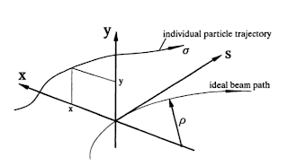
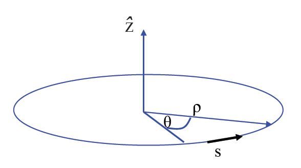
Circular coordinate system [1]
\begin{equation} \vec{R} ~=~ r \vec{x} + y \vec{z}, \end{equation}
where\begin{equation} r ~=~ \rho + x. \end{equation}
These coordinates represent deviations with respect to the ideal design orbit, we assume these deviations to be small; in reality $x$ is in the of order mm. We use the positions $x$ and $y$, and their slopes $x' = \frac{dx}{ds}$ and $y' = \frac{dy}{ds}$.

Circular coordinate system [2]
References
[1] R. Appleby. Beam Dynamics. Cockcroft Lectures 2011
[2] H. Weidemann. Particle Accelerator Physics I: Basic Principles and Linear Beam
Dynamics. Springer, 1999
Wednesday, 16 October 2013
How to Add EBooks to Android Kindle App
Having downloaded the Kindle app for Android, but was having difficulty adding ebooks to my Android's microSD card.
It is easy enough to copy ebooks in their various formats to the kindle folder on an Android external memory, however the Kindle app doesn't always recognise them.
After scouring the internet I found a simple solution;
It is easy enough to copy ebooks in their various formats to the kindle folder on an Android external memory, however the Kindle app doesn't always recognise them.
After scouring the internet I found a simple solution;
- Download the Calibre ebook manager.
- Open Calibre, and use the Add books button (top left corner) to select the required ebooks.

- Use the convert tool to convert the ebooks into .azw3 format, you can also customise the output resolution to suit your own device as well as many other options
- Copy the .azw3 files to your microSD/other storage device, placing them in the kindle/ folder.
- Open the kindle app and use the sync button (top right hand corner) to search for new ebooks. It may take a few minutes to update, depending on the size and number of books added.

Also note that Amazon Prime members can only make use of the free book 'lending' scheme if they are using a Kindle device.
Tuesday, 11 June 2013
The Three Gables
In this instance our Three Gables refer to men of the mathematical world rather than a house in Harrow Weald; Newton, Hamilton and Lagrange.
Let us take the example of the simple pendulum and the three mathematicians' approaches to finding the equations of motion for this dynamical system. The pendulum weight has mass $m$, $\mathbf{x}$ denotes its position vector, $\dot{\mathbf{x}}$ its velocity vector (i.e. $\frac{d(\mathbf{x})}{dt}=\dot{\mathbf{x}}$) and $\mathbf{p}$ is the momentum vector of the pendulum mass.
Approaches
Newton: Relate a force $\mathbf{F}(\mathbf{x}, \dot{\mathbf{x}}, t)$ to the resulting motion using Newton's 2nd law: $F=ma$ or more appropriately $$\frac{d}{dt}m\dot{\mathbf{x}} = \mathbf{F}(\mathbf{x}, \dot{\mathbf{x}}, t).$$
Lagrange: Construct the Lagrangian function $\mathcal{L}(q, \dot{q},t)$ which can normally be given by $\mathcal{L} = T - V$ where $T$ and $V$ are the kinetic and potential energy of the system respectively. The equations of motion are given by the Euler-Lagrange equation: $$ \frac{d\mathcal{L}}{dq_i} - \frac{d}{dt} \left( \frac{d\mathcal{L}}{d\dot{q}_i} \right) = 0.$$
Hamilton: Construct the Hamiltonian function $H(\mathbf{x}, \mathbf{p},t)$, which is a function of a set of conjugate variable pairs. The Hamiltonian contains the dynamics of the system and Hamilton's equations provide the equations of motion: $$ \frac{d\mathbf{x}_i}{dt} = \frac{\partial H}{\partial \mathbf{x}_i}, $$ $$ \frac{d\mathbf{p}_i}{dt} = \frac{\partial H}{\partial \mathbf{p}_i}. $$
1: Newtonian Mechanics
This is the familiar method for most of us. I have dropped the bold font for vectors from here on.
The force on the pendulum mass is given by $F = -kx$ where $k$ is a constant given by $$k = \omega^2 m $$. Thus we can write $$F=-\omega^2 m.$$
Using Newton's 2nd law we get the equation of motion: $$ m \frac{d}{dt} \dot{x} = -m \omega^2 x, $$ which is equivalent to $$ \frac{d^2 x}{dt^2} = - \omega^2x.$$
The solution to this equation is the standard, two constant oscillatory equation: $$ x(t) = x_0 sin(\omega t + \phi_0)$$ where $x_0$ and $\phi_0$ are constants determined by the inital values of $x(t)$ and $\dot{x}(t)$.
2: Lagrangian Mechanics
The pendulum mass has a kinetic energy: $$T = \frac{1}{2} m \dot{x}^2 $$ and a potential energy given by $$V = \frac{1}{2}m \omega^2 x^2.$$
The Lagrangian in this case may be found using $\mathcal{L} = T-V$: $$\mathcal{L} = T-V = \frac{1}{2} m \dot{x}^2 - \frac{1}{2}m \omega^2 x^2. $$
Using the Euler-Lagrange equation: $$ \frac{d\mathcal{L}}{dx_i} - \frac{d}{dt}\left( \frac{d\mathcal{L}}{d\dot{x}_i}\right) = 0.$$
we can do this step by step:
$$ \frac{d\mathcal{L}}{dx_i} = -\omega^2 mx,$$
and:
$$ \frac{d\mathcal{L}}{d\dot{x}_i}=m\dot{x}.$$
Substituting into the Euler-Lagrange equation we have:
$$-\omega^2 m x - \frac{d}{dt}(m\dot{x}) = 0$$
which is equivalent to:
$$\frac{d^2 x}{dt^2} = -\omega^2 x.$$
Which unsurprisingly is equivalent to our Newtonian formulation and has the same standard oscillatory solution.
3: Hamiltonian
Here we need to use the conjugate pair of position $x_i$ and momentum $p_i$. Given the Lagrangian $\mathcal{L}$, the conjugate momentum and Hamiltonian can be derived as follows:
$$p_i = \frac{\partial \mathcal{L}}{\partial \dot{q}_i} = \frac{\partial \mathcal{L}}{\partial \dot{x}_i} = m\dot{x},$$
$$H = \sum_i \dot{q_i}{p_i} - \mathcal{L} = \sum_i \dot{x}_i p_i - \mathcal{L},$$
which leads to:
$$H = \dot{x}p_x - \mathcal{L} = m\dot{x}^2 - \mathcal{L},$$
and finally we have the Hamiltonian:
$$H = \frac{p^2_x}{2m} + \frac{1}{2}m \omega^2 x^2.$$
Using Hamilton's equations:
$$\frac{dx}{dt} = \frac{\partial H}{\partial p_x} = \frac{p_x}{m}, $$
$$\frac{d p_x}{dt}=-\frac{\partial H}{\partial x} = -m \omega^2 x. $$
Note that the last equation is equivalent to Newton's second law.
Remarks
Using Newtonian mechanics, given the function $\mathbf{F}$, we derive the equations of motion, which must be solved to give the explicit dependence of position $x$ (and thus velocity $\dot{x}$) on the independent parameter $t$.
The physics is constructing the form of $\mathbf{F}$ for a gvien system.
Using Lagrangian mechanics the variables $q_i$ can be any convenient set of parameters that describe the system state. We treat $q_i$ and $\dot{q}_i$ as independent variables, despite the fact that they are not. For $n$ degrees of freedom, the Euler-Lagrange equations give us $n$ second-order differential equations.
The physics is constructing the form of $\mathcal{L}$ for a given system.
Using Hamiltonian mechanics a set of conjugate variables that describe the system state must be carefully chosen. We treat the conjugate pair $x,p_x$ as independent variables despite the fact that they are related. For $n$ degrees of freedom, Hamilton's equations give us $2n$ first-order differential equations. Representing the dynamics using first-order differential equations has some advantages when considering linear methods.
The Hamiltonian is conserved if the independent variable does not appear explicitly in the Hamiltonian. This can be shown:
$$\frac{dH}{dt} = \frac{\partial H}{\partial x}\frac{dx}{dt} + \frac{\partial H}{\partial p_x}\frac{d p_x}{dt} + \frac{\partial H}{\partial t}$$
substituting in Hamilton's equations the first two terms cancel:
$$\frac{dH}{dt} = \frac{\partial H}{\partial x}\frac{\partial H}{\partial p_x} + \frac{\partial H}{\partial p_x}\frac{\partial H}{\partial x} + \frac{\partial H}{\partial t} = \frac{\partial H}{\partial t}.$$
If the Hamiltonian does not depend explicitly on $t$, then the Hamiltonian is conserved:
$$\frac{dH}{dt} = \frac{\partial H}{\partial t} = 0.$$
For our system the Hamiltonian could be written: $$H = T + V, $$
which shows that the Hamiltonian appears to be the total energy of the system.
References
[1] Linear Dynamics, Lecture 1: Review of Hamiltonian Mechanics, Andy Wolski, 2006 [Cockcroft lecture series]
[2] Introduction to Beam Dynamics, Rob Appleby, 2011 [Cockcroft lecture series]
Let us take the example of the simple pendulum and the three mathematicians' approaches to finding the equations of motion for this dynamical system. The pendulum weight has mass $m$, $\mathbf{x}$ denotes its position vector, $\dot{\mathbf{x}}$ its velocity vector (i.e. $\frac{d(\mathbf{x})}{dt}=\dot{\mathbf{x}}$) and $\mathbf{p}$ is the momentum vector of the pendulum mass.
Approaches
Newton: Relate a force $\mathbf{F}(\mathbf{x}, \dot{\mathbf{x}}, t)$ to the resulting motion using Newton's 2nd law: $F=ma$ or more appropriately $$\frac{d}{dt}m\dot{\mathbf{x}} = \mathbf{F}(\mathbf{x}, \dot{\mathbf{x}}, t).$$
Lagrange: Construct the Lagrangian function $\mathcal{L}(q, \dot{q},t)$ which can normally be given by $\mathcal{L} = T - V$ where $T$ and $V$ are the kinetic and potential energy of the system respectively. The equations of motion are given by the Euler-Lagrange equation: $$ \frac{d\mathcal{L}}{dq_i} - \frac{d}{dt} \left( \frac{d\mathcal{L}}{d\dot{q}_i} \right) = 0.$$
Hamilton: Construct the Hamiltonian function $H(\mathbf{x}, \mathbf{p},t)$, which is a function of a set of conjugate variable pairs. The Hamiltonian contains the dynamics of the system and Hamilton's equations provide the equations of motion: $$ \frac{d\mathbf{x}_i}{dt} = \frac{\partial H}{\partial \mathbf{x}_i}, $$ $$ \frac{d\mathbf{p}_i}{dt} = \frac{\partial H}{\partial \mathbf{p}_i}. $$
1: Newtonian Mechanics
This is the familiar method for most of us. I have dropped the bold font for vectors from here on.
The force on the pendulum mass is given by $F = -kx$ where $k$ is a constant given by $$k = \omega^2 m $$. Thus we can write $$F=-\omega^2 m.$$
Using Newton's 2nd law we get the equation of motion: $$ m \frac{d}{dt} \dot{x} = -m \omega^2 x, $$ which is equivalent to $$ \frac{d^2 x}{dt^2} = - \omega^2x.$$
The solution to this equation is the standard, two constant oscillatory equation: $$ x(t) = x_0 sin(\omega t + \phi_0)$$ where $x_0$ and $\phi_0$ are constants determined by the inital values of $x(t)$ and $\dot{x}(t)$.
2: Lagrangian Mechanics
The pendulum mass has a kinetic energy: $$T = \frac{1}{2} m \dot{x}^2 $$ and a potential energy given by $$V = \frac{1}{2}m \omega^2 x^2.$$
The Lagrangian in this case may be found using $\mathcal{L} = T-V$: $$\mathcal{L} = T-V = \frac{1}{2} m \dot{x}^2 - \frac{1}{2}m \omega^2 x^2. $$
Using the Euler-Lagrange equation: $$ \frac{d\mathcal{L}}{dx_i} - \frac{d}{dt}\left( \frac{d\mathcal{L}}{d\dot{x}_i}\right) = 0.$$
we can do this step by step:
$$ \frac{d\mathcal{L}}{dx_i} = -\omega^2 mx,$$
and:
$$ \frac{d\mathcal{L}}{d\dot{x}_i}=m\dot{x}.$$
Substituting into the Euler-Lagrange equation we have:
$$-\omega^2 m x - \frac{d}{dt}(m\dot{x}) = 0$$
which is equivalent to:
$$\frac{d^2 x}{dt^2} = -\omega^2 x.$$
Which unsurprisingly is equivalent to our Newtonian formulation and has the same standard oscillatory solution.
3: Hamiltonian
Here we need to use the conjugate pair of position $x_i$ and momentum $p_i$. Given the Lagrangian $\mathcal{L}$, the conjugate momentum and Hamiltonian can be derived as follows:
$$p_i = \frac{\partial \mathcal{L}}{\partial \dot{q}_i} = \frac{\partial \mathcal{L}}{\partial \dot{x}_i} = m\dot{x},$$
$$H = \sum_i \dot{q_i}{p_i} - \mathcal{L} = \sum_i \dot{x}_i p_i - \mathcal{L},$$
which leads to:
$$H = \dot{x}p_x - \mathcal{L} = m\dot{x}^2 - \mathcal{L},$$
and finally we have the Hamiltonian:
$$H = \frac{p^2_x}{2m} + \frac{1}{2}m \omega^2 x^2.$$
Using Hamilton's equations:
$$\frac{dx}{dt} = \frac{\partial H}{\partial p_x} = \frac{p_x}{m}, $$
$$\frac{d p_x}{dt}=-\frac{\partial H}{\partial x} = -m \omega^2 x. $$
Note that the last equation is equivalent to Newton's second law.
Remarks
Using Newtonian mechanics, given the function $\mathbf{F}$, we derive the equations of motion, which must be solved to give the explicit dependence of position $x$ (and thus velocity $\dot{x}$) on the independent parameter $t$.
The physics is constructing the form of $\mathbf{F}$ for a gvien system.
Using Lagrangian mechanics the variables $q_i$ can be any convenient set of parameters that describe the system state. We treat $q_i$ and $\dot{q}_i$ as independent variables, despite the fact that they are not. For $n$ degrees of freedom, the Euler-Lagrange equations give us $n$ second-order differential equations.
The physics is constructing the form of $\mathcal{L}$ for a given system.
Using Hamiltonian mechanics a set of conjugate variables that describe the system state must be carefully chosen. We treat the conjugate pair $x,p_x$ as independent variables despite the fact that they are related. For $n$ degrees of freedom, Hamilton's equations give us $2n$ first-order differential equations. Representing the dynamics using first-order differential equations has some advantages when considering linear methods.
The Hamiltonian is conserved if the independent variable does not appear explicitly in the Hamiltonian. This can be shown:
$$\frac{dH}{dt} = \frac{\partial H}{\partial x}\frac{dx}{dt} + \frac{\partial H}{\partial p_x}\frac{d p_x}{dt} + \frac{\partial H}{\partial t}$$
substituting in Hamilton's equations the first two terms cancel:
$$\frac{dH}{dt} = \frac{\partial H}{\partial x}\frac{\partial H}{\partial p_x} + \frac{\partial H}{\partial p_x}\frac{\partial H}{\partial x} + \frac{\partial H}{\partial t} = \frac{\partial H}{\partial t}.$$
If the Hamiltonian does not depend explicitly on $t$, then the Hamiltonian is conserved:
$$\frac{dH}{dt} = \frac{\partial H}{\partial t} = 0.$$
For our system the Hamiltonian could be written: $$H = T + V, $$
which shows that the Hamiltonian appears to be the total energy of the system.
References
[1] Linear Dynamics, Lecture 1: Review of Hamiltonian Mechanics, Andy Wolski, 2006 [Cockcroft lecture series]
[2] Introduction to Beam Dynamics, Rob Appleby, 2011 [Cockcroft lecture series]
Monday, 10 June 2013
LaTeX in Blogger
Sunday, 5 May 2013


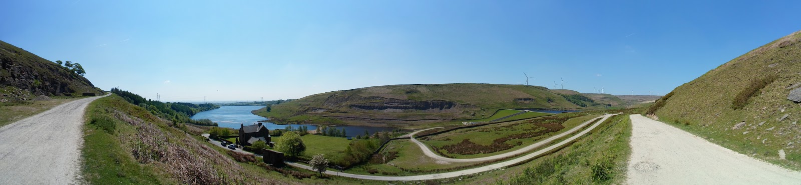
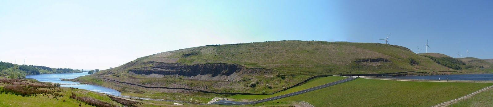


United Nations office in Geneva

The Assembly Hall - the largest room in the Palace of Nations.

The Human Rights and Alliance of Civilisations Room, decorated by famous artist Miquel Barcelo - see how the ceiling was made by clicking here.


The Council Chamber, where many important historical negotiations have taken place, with murals by Jose Maria Sert.

Peak District: Edale (March 2012)
Members of the NGACDT visited Huddersfield in March 2012. Anna Kolano had the idea of going for a hike in the peak district.


Panos is visible taking a photograph to the right of the middle. The rest of the group are sat on a large rock to the right of the image.

The group is visible on the left of the image.

Anna is visible to the right of the image, and Rob, Amanda and Manu are visible on the left.

The small dots in the sky to the left are paragliders.
CERN 2012
A few images taken at The European Centre for Nuclear Research (CERN) in the summer of 2012.

The view from the LHCb flat in Meyrin. The Jura mountains are visible on the right.

The magnet testing facility at point 2.

The main CERN site in Meyrin. The CERN Globe is visible over the farms.

The CERN Prevessin site entrance. The Jura mountains are visible in the background.

Prevessin site entrance.

Magnet testing facility.

Magnet testing facility.

Magnet testing facility. The large blue apparatus in an LHC dipole.
Geneva 2012
A few panoramic images taken around Lake Geneva.

Inside the Ariana Museum.

Lake Geneva - note the parrot sat on the white-shirted man's shoulder.

Lake Geneva.

Lake Geneva with the Jet D'eau.

Lake Geneva with the Jet D'eau and Mont Blanc.

Lake Geneva with the Jet D'eau and Mont Blanc.

Lake Geneva.

Outside the science museum in Parc du Lac.

Outside the science museum in Parc du Lac.
Subscribe to:
Posts (Atom)